Lift Test Calibration#
Introduction#
You may have heard of the phrase “All models are wrong but some are useful.” This is true in many areas, and it’s likely that after the first attempt, you haven’t yet created a model that can accurately determine your true attribution. Even if you have, how can you be sure? We create models to understand the attribution of our marketing channels, but it appears that even then, we can’t always rely on what the models tell us.
In order to ensure that our models are decomposing correctly, we can use various testing methods to gather real-world data and compare it with our models. This will help us to identify any discrepancies and improve the decomposition accuracy of our models.
Today, we will explore a new way to integrate experiments into pymc-marketing. This will bring us closer to accurate representations of real-world values and improve the estimates generated by our models.
When are lifts test useful?#
In some situations, all of the relevant experiment spend data is captured within historical data that you will including in your training set. In these cases, a valid approach could be to simply train your MMM on all available data (including experiment and non-experiment periods) in order to optimally inform you about model parameters and ultimately get better insights. However there are a number of situations when this approach will not be appropriate.
Imagine your online advertising platform gave you additional credit. You decide to spend this credit by increasing activity on a digital ad channel and you want to use this as a way to evaluate the uplift. In this situation, you will have increased the level of advertising taking place, but this ‘increased spend’ is not charged to your invoice. So unless your data pipeline is really on point, your spend data will not accurately reflect the level of effective spend.
You want to run a test on TV. In that case, you probably have to pay months before the test takes place or the commercial is aired. So, your spending may be in February and the action in March, but during the period of the experiment itself, there is no spending. Here, the spend may well be contained in your training data, but the time lag between the spend and the advertising takes place is very high. So the adstock function which accommodates short term lag effects may not adequately capture longer term lags such as this.
You are experimenting with discounts or promotions. These might be quantifiable, but not show up in your traditional media spend channels and so your experimentation may not be captured by your MMM.
These are just a few examples where lift tests can be useful. In these cases, you can use the results of the lift test to adjust the model parameters and improve the accuracy of the model.
Requirements#
Today, we won’t be discussing how to conduct lift tests, but instead, we will focus on their utilization. If you wish to acquire knowledge on how to generate results that are compatible with your MMM models, you can check out CausalPy for conducting experiments, such as using Interrupted Time Series for lift tests with no control groups.
Goal#
After reading this notebook, you will have gained the necessary expertise to incorporate the results (detected uplift from your experiments) into our regressive model.
This notebook will display using the add_lift_test_measurements method of MMM and its workflow:
Build model:
mmm.build_model(X, y)Add lift measurements:
mmm.add_lift_test_measurements(df_lift_test)Sample posterior:
mmm.fit(X, y)
This is a case study of two correlated channels to see how lift tests help distinguish the channel effects.
import warnings
from functools import partial

import arviz as az
import matplotlib.pyplot as plt
import numpy as np
import pandas as pd
import pymc as pm
import seaborn as sns

from pymc_marketing.mmm import GeometricAdstock, LogisticSaturation
from pymc_marketing.mmm.multidimensional import MMM
from pymc_marketing.mmm.transformers import logistic_saturation
OMP: Info #276: omp_set_nested routine deprecated, please use omp_set_max_active_levels instead.
/Users/carlostrujillo/Documents/GitHub/pymc-marketing/pymc_marketing/mmm/multidimensional.py:216: FutureWarning: This functionality is experimental and subject to change. If you encounter any issues or have suggestions, please raise them at: https://github.com/pymc-labs/pymc-marketing/issues/new
  warnings.warn(warning_msg, FutureWarning, stacklevel=1)
warnings.filterwarnings("ignore")

az.style.use("arviz-darkgrid")
plt.rcParams["figure.figsize"] = [12, 7]
plt.rcParams["figure.dpi"] = 100

%config InlineBackend.figure_format = "retina"
seed = sum(map(ord, "Lift tests help distinguish channel effects"))
rng = np.random.default_rng(seed)
Generate Correlated Spends and Model Target#
First we’ll generate synthetic data for two channels with completely correlated spends.
n_dates = 52
dates = pd.date_range(start="2024-01-01", periods=n_dates, freq="W-MON")
spend_rv = pm.Uniform.dist(lower=0.1, upper=1, size=n_dates)
spend = pm.draw(spend_rv, random_seed=rng)
spend1 = spend / spend.max()
spend2 = spend - 0.05
spend2 /= spend2.max()
df = pd.DataFrame(
    {
        "date": dates,
        "channel 1": spend1,
        "channel 2": spend2,
    }
)

ax = df.set_index("date").plot(ylabel="channel spend");
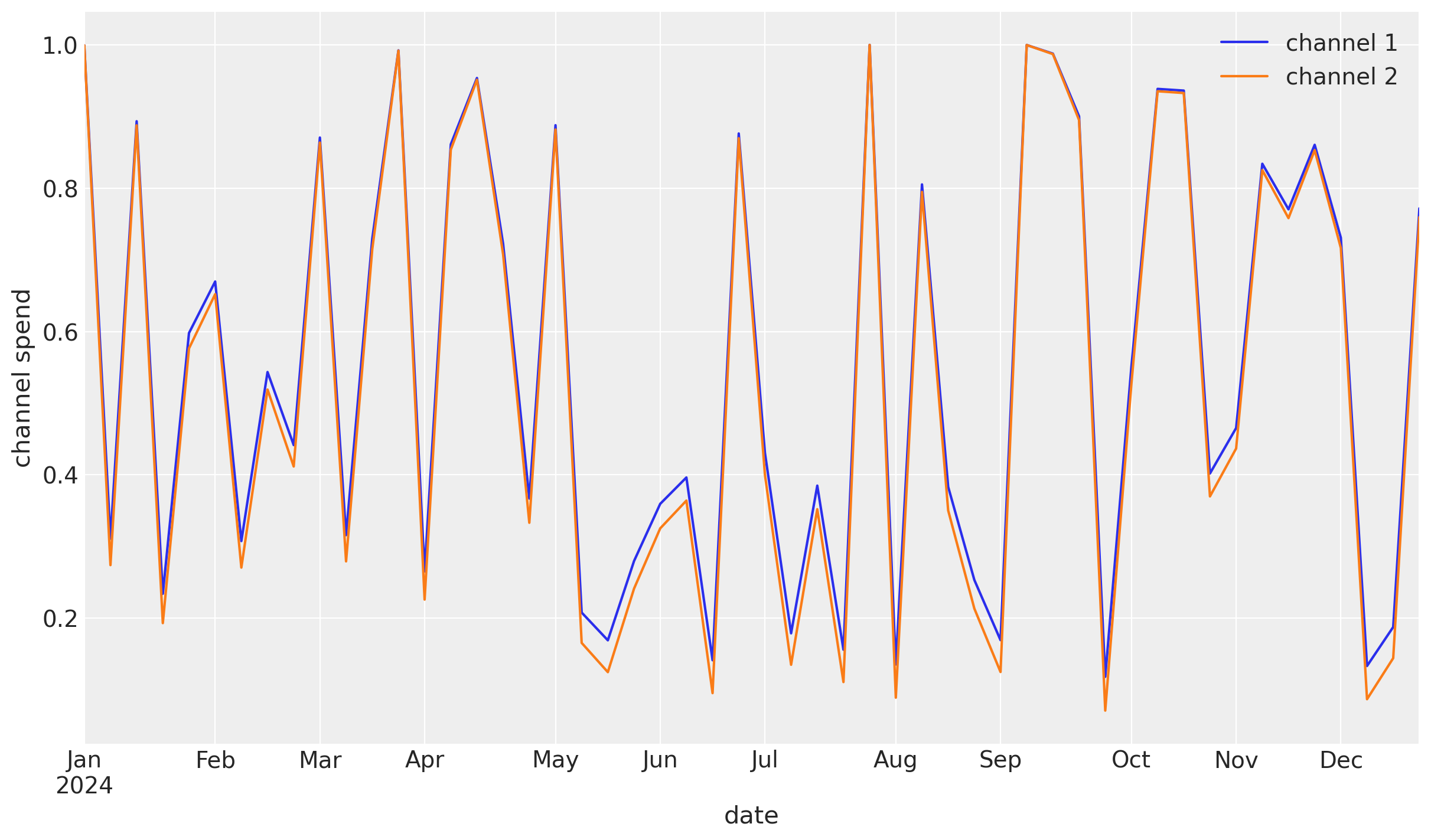
Note
For this example, the synthetic spend data is not produced in a overly realistic manner. However, we have normalized the maxmium spend to 1 for each channel to mimmick data pre-processing that typically takes place in a pymc-marketing workflow.
We can double check that the to channels are perfectly correlated.
df.filter(regex="channel").corr()
| channel 1 | channel 2 | |
|---|---|---|
| channel 1 | 1.0 | 1.0 |
| channel 2 | 1.0 | 1.0 |
We use the MMM class to specify our model just as usual.
mmm = MMM(
    date_column="date",
    target_column="y",
    channel_columns=["channel 1", "channel 2"],
    adstock=GeometricAdstock(l_max=6).set_dims_for_all_priors("channel"),
    saturation=LogisticSaturation().set_dims_for_all_priors("channel"),
)
For this constructed example, we will set parameter of the model with the pm.do operator and take a random sample of the target variable. The fixed parameters are below which we will try to recover.
At this point, a model has not been fit. However, we have created our data set to fit our model on.
true_lam_c1 = 10
true_beta_c1 = 0.55

true_lam_c2 = 1.5
true_beta_c2 = 1.0

true_params = {
    "adstock_alpha": np.array([0.5, 0.5]),
    "saturation_lam": np.array([true_lam_c1, true_lam_c2]),
    "saturation_beta": np.array([true_beta_c1, true_beta_c2]),
    "intercept_contribution": 0.5,
    "y_sigma": 0.25,
}
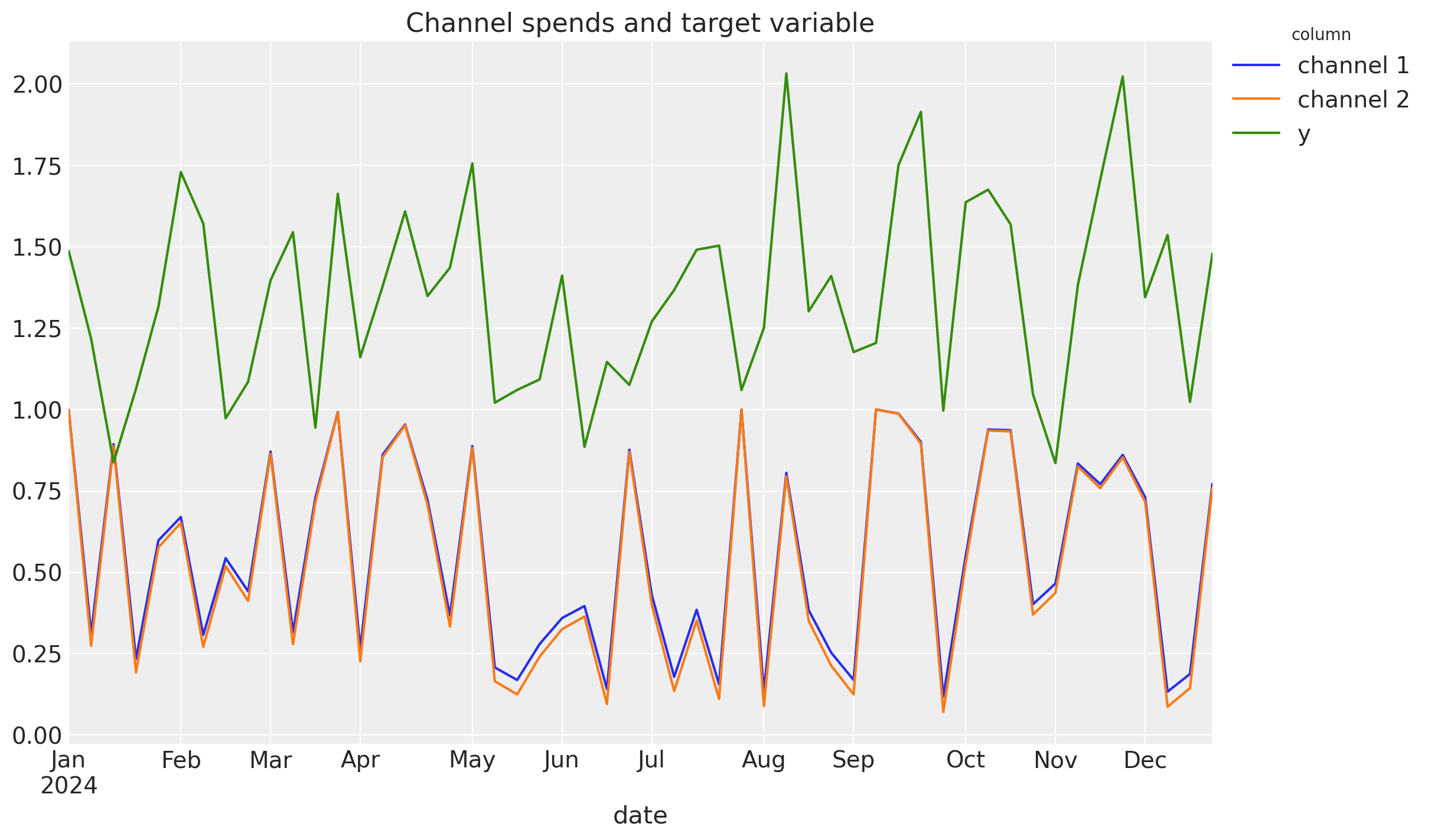
df["y"] = np.ones(n_dates)
ax = df.set_index("date").plot(ylabel="", title="Channel spends and target variable")
ax.legend(bbox_to_anchor=(1.0, 1.05), title="column");
X = df.drop(columns=["y"])
y = df["y"]
mmm.build_model(X=X, y=y)
mmm.add_original_scale_contribution_variable(["channel_contribution"])
Indistinguishable Parameter Estimates#
In order to show the trouble that completely correlated channels provides, let’s fit the model
fit_kwargs = {"nuts_sampler": "numpyro", "random_seed": rng}

idata_without = mmm.fit(X, y, **fit_kwargs)
There were 10 divergences after tuning. Increase `target_accept` or reparameterize.
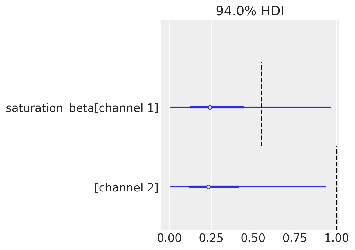
Since the spends are completely correlated, there is no way to distinguish the parameters. Not only that, but the parameter estimates are not close to actuals.
ax = az.plot_forest(idata_without, var_names=["saturation_lam"], combined=True)[0]

plot_true_value(true_lam_c1, "channel 1", ax=ax, split=0.4)
plot_true_value(true_lam_c2, "channel 2", ax=ax, split=0.4);

ax = az.plot_forest(idata_without, var_names=["saturation_beta"], combined=True)[0]

plot_true_value(true_beta_c1, "channel 1", ax=ax, split=0.4)
plot_true_value(true_beta_c2, "channel 2", ax=ax, split=0.4);
We can also witness that while the actual saturation curves are different (because we specified the true parameters for each channel), the MMM is unable to distinguish between the two channels.
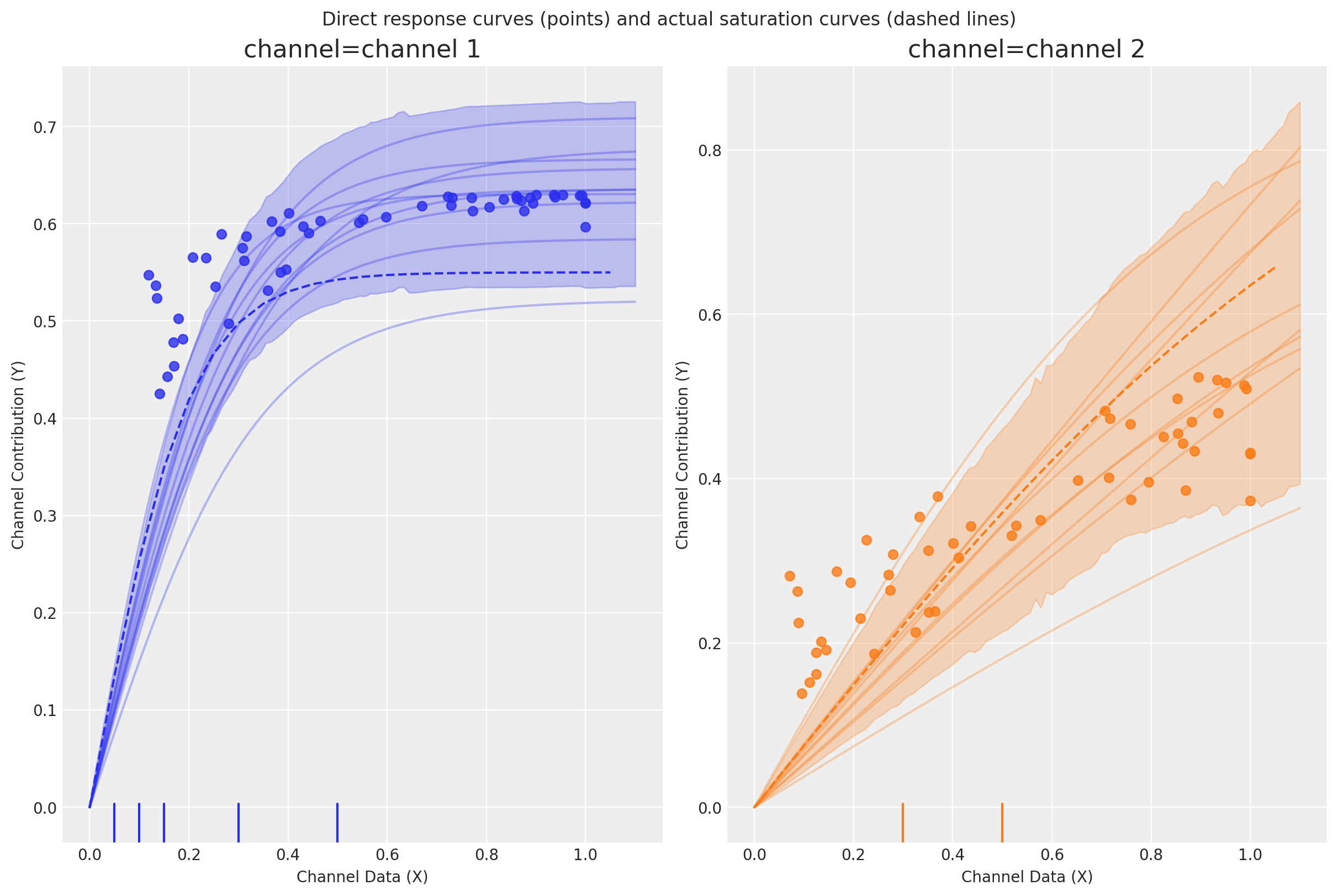
We can show this below by plotting the actual saturation curves (lines) and the direct response curves (points).
Direct response curves
Plots the direct contribution curves for each marketing channel. The term “direct” refers to the fact we plot costs vs immediate returns and we do not take into account the lagged effects of the channels e.g. adstock transformations. And so these curves will actually consist of a series of points, each representing the direct contribution of a spend level.
curve = mmm.saturation.sample_curve(
    mmm.idata.posterior[["saturation_beta", "saturation_lam"]], max_value=1.1
)
fig, axes = mmm.plot.saturation_curves(
    curve,
    original_scale=True,
    n_samples=10,
    hdi_probs=0.85,
    random_seed=rng,
    subplot_kwargs={"figsize": (12, 8), "ncols": 2},
    rc_params={
        "xtick.labelsize": 10,
        "ytick.labelsize": 10,
        "axes.labelsize": 10,
        "axes.titlesize": 10,
    },
)


def plot_actual_curves(
    axes_array: np.ndarray, linestyle: str | None = None
) -> np.ndarray:
    axes_array[0].plot(xx, c1_curve, label="channel 1", color="C0", linestyle=linestyle)
    axes_array[1].plot(xx, c2_curve, label="channel 2", color="C1", linestyle=linestyle)

    return axes_array


def plot_reference(ax: plt.Axes) -> plt.Axes:
    ax.plot(xx, xx, label="y=x", color="black", linestyle="--")

    return ax


axes = np.ravel(axes)
plot_actual_curves(axes, linestyle="dashed")
fig.suptitle(
    "Direct response curves (points) and actual saturation curves (dashed lines)"
);
Sampling: []

We can see that the true but latent saturation curves (dashed lines) for each channel are different, but that the the MMM is unable to distinguish that the saturation curves for each channel (points) are different. And this is because the spends are perfectly correlated.
Let’s see if we can improve upon this by adding lift test measurements.
Note
In order to avoid confusion with the plot above, the actual saturation curves are represented by the dashed lines, while the direct contribution curves are represented by the points. If lift tests can help us in this situation of high spend correlation, then we should be able to detect this by: a) achieving better parameter estimates, and b) correspondingly, getting better estimates of the saturation curves.
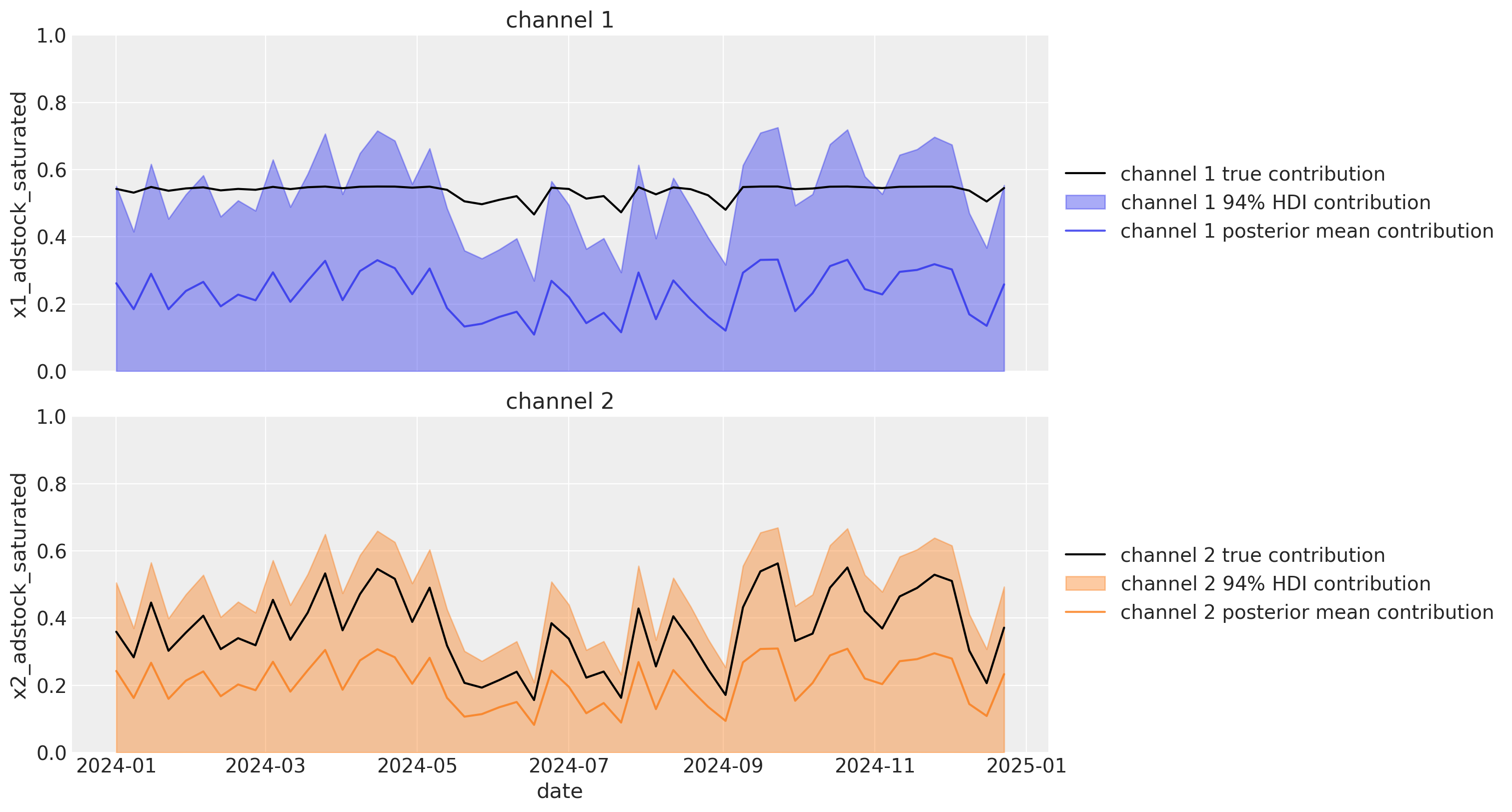
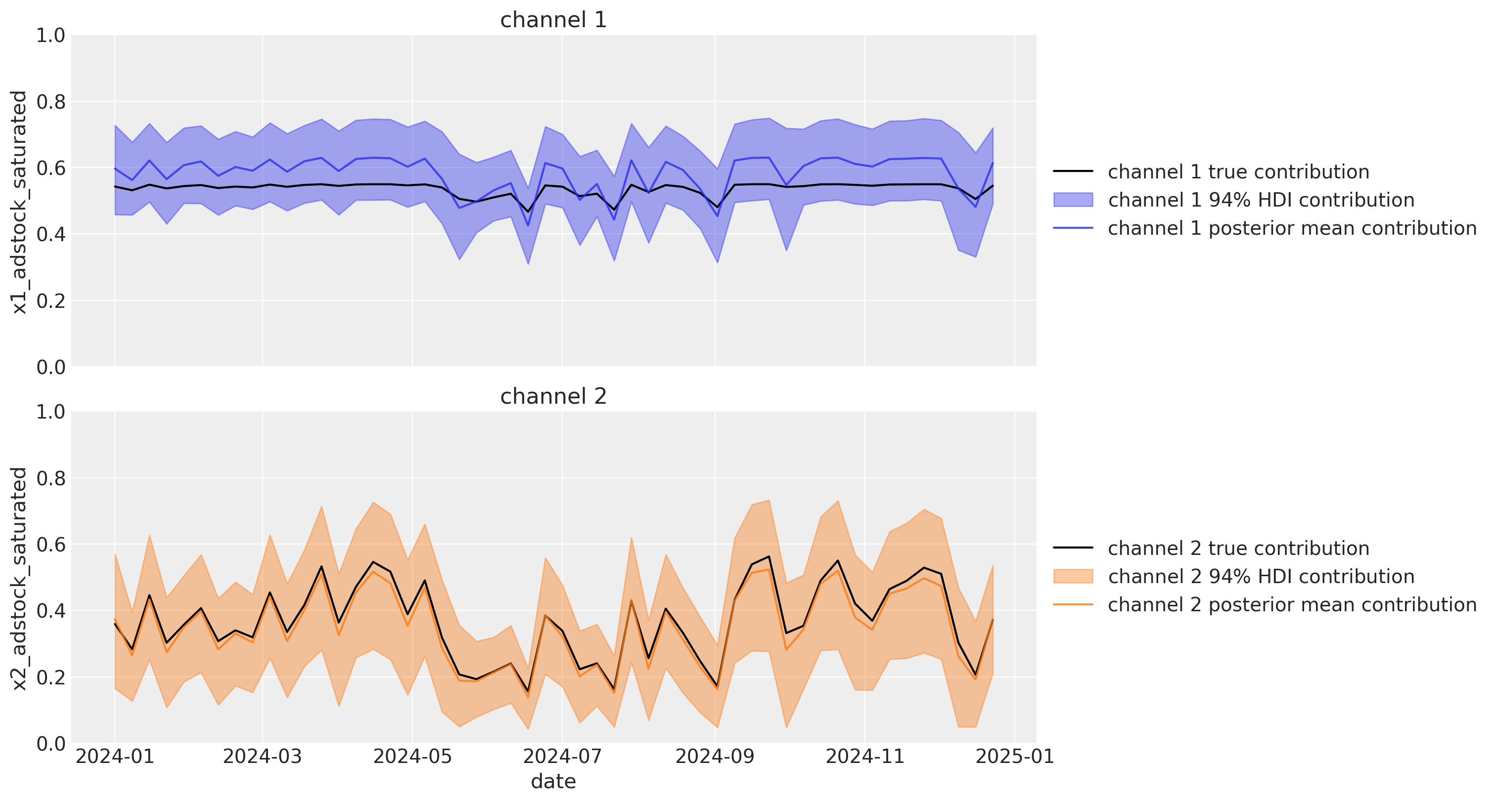
We can also visualize the channel contributions over time. The wide HDI’s in the plot below shows that we have considerable uncertainty in the channel contributions. We can also see that the posterior means of the channel contributions are quite far off the mark of the actual channel contributions. Again, these true channel contributions are only known to us in this synthetic data example and would not be available to us in a real world scenario.
plot_channel_contributions(mmm, df)
About Lift Tests#
In a lift study, one temporarily changes the budget of a channel for a fixed period of time, and then uses some method (for example CausalPy) to make inference about the change in sales directly caused by the adjustment.
A lift test is characterized by:
channel: the channel that was testedx: pre-test channel spenddelta_x: change made toxdelta_y: inferred change in sales due todelta_xsigma: standard deviation ofdelta_y
An experiment characterized in this way can be viewed as two points on the saturation curve for the channel. Accordingly, lift test calibration is implemented by adding a term to the model likelihood, that makes the channel saturation curve (the contribution as a function of spend) align with the test observation.
def create_lift_test_from_actual_curve(
    channel: str, x: float, delta_x: float, sigma: float
) -> dict[str, float]:
    curve_fn = c1_curve_fn if channel == "channel 1" else c2_curve_fn
    delta_y = curve_fn(x + delta_x) - curve_fn(x)

    return {
        "channel": channel,
        "x": x,
        "delta_x": delta_x,
        "delta_y": delta_y,
        "sigma": sigma,
    }
df_lift_test = pd.DataFrame(
    [
        # Channel x1
        create_lift_test_from_actual_curve("channel 1", 0.05, 0.05, 0.05),
        create_lift_test_from_actual_curve("channel 1", 0.15, 0.05, 0.05),
        create_lift_test_from_actual_curve("channel 1", 0.3, -0.05, 0.05),
        # Channel x2
        create_lift_test_from_actual_curve("channel 2", 0.5, 0.05, 0.10),
    ]
)

df_lift_test
| channel | x | delta_x | delta_y | sigma | |
|---|---|---|---|---|---|
| 0 | channel 1 | 0.05 | 0.05 | 0.119459 | 0.05 |
| 1 | channel 1 | 0.15 | 0.05 | 0.069545 | 0.05 |
| 2 | channel 1 | 0.30 | -0.05 | -0.031276 | 0.05 |
| 3 | channel 2 | 0.50 | 0.05 | 0.032236 | 0.10 |
Let’s visualise the lift test results to get an understanding of how they can better inform the model parameters - specifically the saturation curve parameters.

fig, ax = plt.subplots(1, 1, figsize=(12, 5))
plot_lift_test_triangles(df_lift_test, ax)
ax.set_title("lift test showing different diminishing returns")
ax.set_ylabel("change in contribution")
ax.set_xlabel("x")
plt.tight_layout();
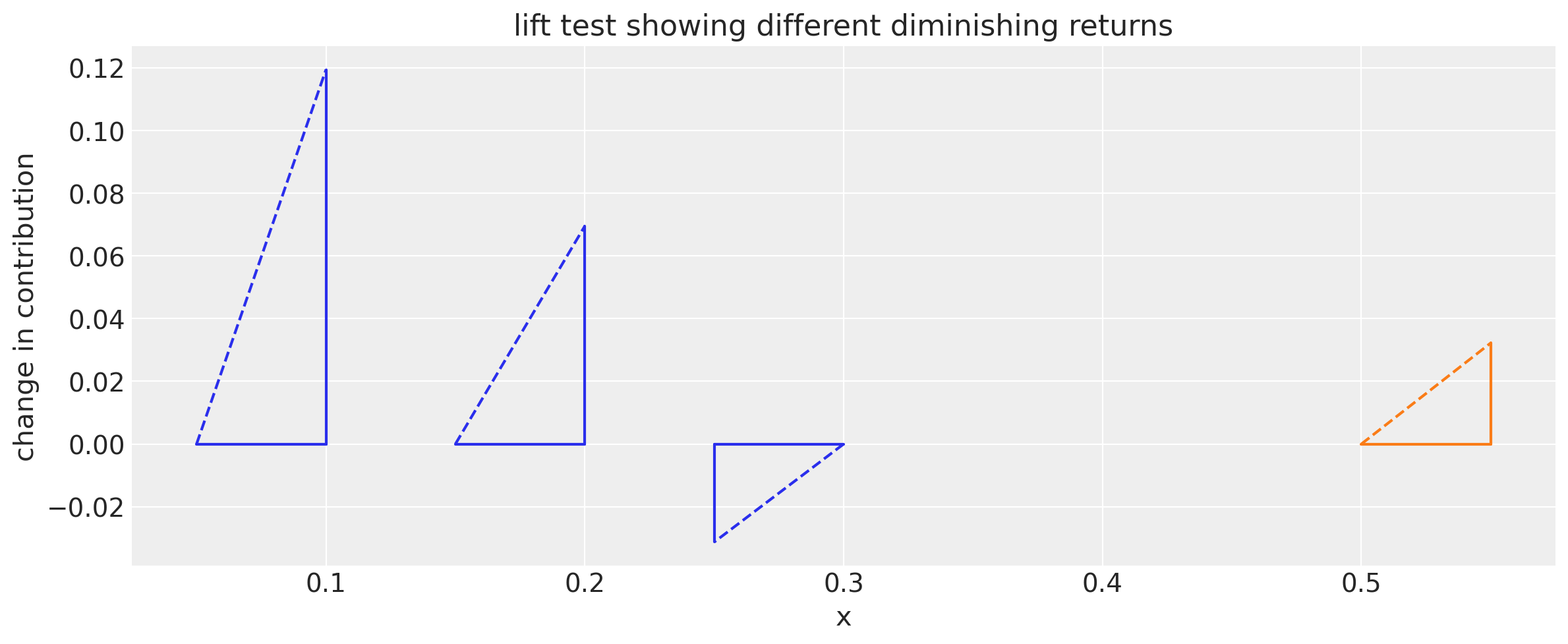
The top plot shows the results superimposed upon the actual saturation curves. In a real situation we would not know the actual saturation curves, but the plot here is incuded to aid understanding of what is taking place.
The bottom plot shows the same results but at y=0, focussing on the fact that we are only observing the change in contribution. This is more true of the partial knowledge you’d have in a real situation.
Lift tests are visualized with the triangles. The base of the triangle shows the change in the spend and height of triangle is change in contribution.
While we only have the information in the bottom plot, the top plot shows how the lift test information can be used to help better estimate the saturation curves.
For example, just from the lift tests (bottom triangles) we can see that channel 2 is slower to saturate than channel 1 because we get a higher change in contribution at higher spend levels.
Note
The first 2 lift tests on channel 1 involved increasing the spend on that channel. However the third lift test on channel 1 involved a decrease in the spend. It is useful to be able to consider both increases and decreases in spend in lift tests. And there is nothing getting in the way of making this decrease even more extreme by temporarily setting the spend to zero.
Add Lift Tests to Model#
Having created a MMM model instance, mmm and built it using the build_model method or fit with fit method, we can add lift test results to the model using the add_lift_test_measurments method.
First, let’s take a look at the model graph before adding the lift test measurements.
mmm.graphviz()

And now we’ll add the lift test measurements to the model and see how our model graph has changed.
mmm.add_lift_test_measurements(df_lift_test)
mmm.graphviz()

We can see the model graph is modified with new observation for our lift measurements. The observation distribution is assumed to be Gamma as each saturation curve is monotonically increasing given a set of parameters.
In short, this works by providing a new likelihood term of the form
where:
\(|\Delta_y|\) is the observed absolute change in contribution - as estimate from the lift test.
\(|\tilde{\text{lift}}|\) is the absolute change in contribution as estimated by the model, i.e. based on the parameterized saturation curve.
\(\sigma\) is the standard deviation of the increase in \(\Delta_y\) of lift test. That is, we have uncertainty in the result of the lift test, and \(\sigma\) represents the standard deviation of this uncertainty.
How Lift Tests Are Implemented in PyMC
While the add_lift_test_measurements method handles all of this automatically in pymc-marketing, understanding the implementation mechanics is valuable. This section provides a step-by-step guide to how lift tests are integrated into the model.
Why the Gamma Distribution?
The choice of a Gamma distribution for the lift test likelihood is deliberate and mathematically motivated:
Saturation curves are monotonically increasing: Given a fixed set of parameters, as spend increases, contribution increases (or stays the same, but never decreases). This is a fundamental property of saturation functions used in MMM.
Lifts must be non-negative: The change in contribution from a change in spend must be non-negative (when taking absolute values).
Gamma is natural for positive quantities: The Gamma distribution is defined only for positive real numbers, making it a natural choice for modeling non-negative lift values.
Handling spend decreases: By taking absolute values of both the observed and predicted lift (\(|\Delta_y|\) and \(|\tilde{\text{lift}}|\)), we can handle both increases and decreases in spend. A decrease in spend from \(x\) to \(x - \delta\) produces the same (absolute) lift magnitude as an increase from \(x - \delta\) to \(x\).
While one could alternatively use a Normal distribution with absolute values, the Gamma distribution is more theoretically appropriate for strictly positive quantities and often provides better numerical stability in practice.
Implementation Algorithm
The following steps outline how lift test observations are added to a PyMC model:
Step 1: Scale the Lift Test Data
MMMs typically work with scaled/normalized data internally (e.g., using max scaling where each variable is divided by its maximum value). Lift tests, however, are specified in original units. Therefore, the first step is to transform the lift test measurements to match the model’s internal scale:
# Pseudo-code
# Scale channel-related measurements (x, delta_x)
x_scaled = channel_scaler.transform(x)
delta_x_scaled = channel_scaler.transform(x + delta_x) - x_scaled

# Scale target-related measurements (delta_y, sigma)
delta_y_scaled = target_scaler.transform(delta_y)
sigma_scaled = target_scaler.transform(sigma)
This ensures that the lift test observations are compatible with the model’s internal representation of channels and target.
NOTE: This is done internally, users do not implement this step.
Step 2: Map DataFrame Coordinates to Model Indices
Each row in the lift test DataFrame corresponds to specific coordinates in the model. We need to map these coordinate values to their integer indices in the model:
# Example: if df has channel values ["channel_1", "channel_2", "channel_1"]
# and the model coords are {"channel": ["channel_1", "channel_2", "channel_3"]}
# then we map to indices: [0, 1, 0]

indices = {}
for dim in required_dims:  # e.g., ["channel"] or ["channel", "geo"]
    lift_values = df_lift_test[dim].values
    model_coords = model.coords[dim]
    # Find index of each lift test value in model coordinates
    indices[dim] = [model_coords.index(val) for val in lift_values]
This coordinate mapping is essential for extracting the correct parameter values for each lift test.
Note: For a simple national-level MMM (with only a “channel” dimension), this step is straightforward—you’re just mapping channel names to indices. The complexity of this step increases for multi-dimensional models (e.g., channel × geo × product) where each lift test must be mapped across multiple coordinate dimensions simultaneously.
Step 3: Extract Parameter Values for Each Lift Test
For each lift test, we need to extract the specific parameter values that apply to that test’s coordinates. For example, if testing “channel_1”, we need saturation_lam[0] and saturation_beta[0]:
# Create an indexer function that extracts parameters at specific coordinates
def get_parameter_at_indices(param_name):
    param = model[param_name]  # e.g., saturation_lam with dims=("channel",)
    dims = model.named_vars_to_dims[param_name]  # e.g., ("channel",)

    # Index into parameter using the coordinate indices
    idx = tuple([indices[dim] for dim in dims])
    return param[idx]

# Example: for lift tests on channels [0, 1, 0]
# get_parameter_at_indices("saturation_lam") returns [lam[0], lam[1], lam[0]]
Step 4: Evaluate the Saturation Curves
Now we compute the model’s prediction for each lift test by evaluating the saturation function at two points: before and after the spend change:
# Convert lift test data to PyTensor tensors
x_before = pt.as_tensor_variable(df_lift_test["x_scaled"])
x_after = x_before + pt.as_tensor_variable(df_lift_test["delta_x_scaled"])

# Define saturation curve evaluation with extracted parameters
def saturation_curve(x):
    return saturation_function(
        x,
        lam=get_parameter_at_indices("saturation_lam"),
        beta=get_parameter_at_indices("saturation_beta"),
    )

# Compute model-estimated lift: the key computation
model_estimated_lift = saturation_curve(x_after) - saturation_curve(x_before)
This model_estimated_lift is a PyTensor expression that depends on the model parameters, so it becomes part of the computational graph and will be different for each MCMC sample.
Step 5: Add the Likelihood Term
Finally, we add a Gamma observation to the PyMC model that links the model’s predicted lift to the empirically observed lift:
with model:
    pm.Gamma(
        name="lift_measurements",
        mu=pt.abs(model_estimated_lift),  # model's prediction
        sigma=df_lift_test["sigma_scaled"],  # measurement uncertainty
        observed=pt.abs(df_lift_test["delta_y_scaled"]),  # observed data
    )
This creates an additional likelihood term in the model. During MCMC sampling, the sampler will try to find parameter values that not only fit the main time series data but also produce saturation curves consistent with the lift test observations.
Summary
Lift tests act as additional observations of the saturation curve that constrain the model parameters during inference. Instead of only learning from the historical time series (which may have limited variation or correlated channels), the model also learns from controlled experiments that directly probe the saturation curve at specific points.
This is particularly valuable when:
Channels are highly correlated in historical data (as in this notebook’s example)
You want to validate that the model’s saturation curves match real-world behavior
Historical data has limited variation in spend levels for certain channels
By adding lift test measurements, you’re essentially saying: “I know that at spend level \(x\) for this channel, a change of \(\Delta x\) produces a contribution change of approximately \(\Delta y\).” This directly informs the saturation curve parameters and helps the model distinguish between otherwise confounded effects.
We can refit the model but with the lift tests included
idata_with = mmm.fit(X, y, **fit_kwargs)
The model gets shaped by the lift test measurements and the response curves begin to separate!
curve = mmm.saturation.sample_curve(
    mmm.idata.posterior[["saturation_beta", "saturation_lam"]], max_value=1.1
)
fig, axes = mmm.plot.saturation_curves(
    curve,
    original_scale=True,
    n_samples=10,
    hdi_probs=0.85,
    random_seed=rng,
    subplot_kwargs={"figsize": (12, 8), "ncols": 2},
    rc_params={
        "xtick.labelsize": 10,
        "ytick.labelsize": 10,
        "axes.labelsize": 10,
        "axes.titlesize": 10,
    },
)


def plot_lift_test_rugs_on_axes(
    axes_array: np.ndarray, df: pd.DataFrame, height: float = 0.05
) -> np.ndarray:
    # Channel 1 lift tests on first axis
    idx_c1 = df["channel"] == "channel 1"
    if idx_c1.any():
        plot_channel_rug(df.loc[idx_c1], color="C0", ax=axes_array[0], height=height)

    # Channel 2 lift tests on second axis
    idx_c2 = df["channel"] == "channel 2"
    if idx_c2.any():
        plot_channel_rug(df.loc[idx_c2], color="C1", ax=axes_array[1], height=height)

    return axes_array


axes = np.ravel(axes)
plot_actual_curves(axes, linestyle="dashed")
plot_lift_test_rugs_on_axes(axes, df_lift_test)
fig.suptitle(
    "Direct response curves (points) and actual saturation curves (dashed lines)"
);
Sampling: []

The ‘rug’ marks in the plot above show the initial channel spend before the lift test.
Below we show the (currently modest) changes in the saturation parameter estimates. The idea is that as we add more lift tests (see later), we can better estimate the saturation curves.
data = [idata_without, idata_with]
model_names = ["without lift tests", "with lift tests"]

ax = plot_comparison(data, model_names, "saturation_lam")
plot_true_value(true_lam_c1, "channel 1", ax)
plot_true_value(true_lam_c2, "channel 2", ax);

ax = plot_comparison(data, model_names, "saturation_beta")
plot_true_value(true_beta_c1, "channel 1", ax)
plot_true_value(true_beta_c2, "channel 2", ax);

Careful examination of these 2 plots shows that the posterior mean has shifted closer to the true parameter value and/or the HDI is shrinking, indicating improved precision of our estimates.
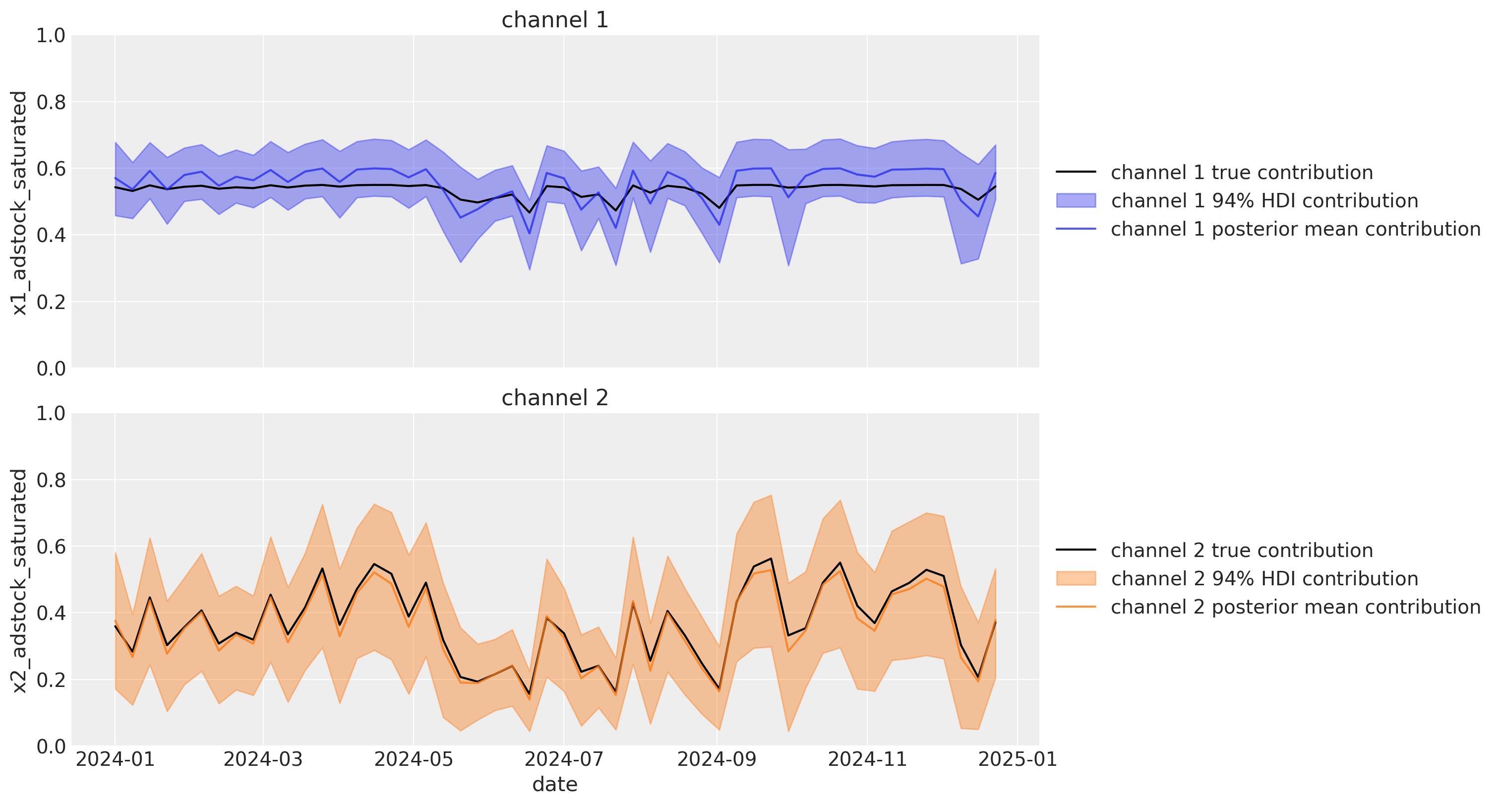
Let’s return to our estimated channel contributions over time. The HDI’s are narrower than before, indicating that we have reduced the uncertainty in our channel contribution estimates. Even more impressively, the posterior mean estimates are now much closer to the actual channel contributions.
plot_channel_contributions(mmm, df)

Add Additional Lift Tests#
We can add even more lift tests.
They can either all be added at one time or separately.
df_additional_lift_test = pd.DataFrame(
    [
        # More for Channel x1
        create_lift_test_from_actual_curve("channel 1", 0.1, 0.05, sigma=0.01),
        create_lift_test_from_actual_curve("channel 1", 0.5, 0.05, sigma=0.01),
        # More for channel x2
        create_lift_test_from_actual_curve("channel 2", 0.3, 0.05, sigma=0.01),
    ]
)

df_additional_lift_test
| channel | x | delta_x | delta_y | sigma | |
|---|---|---|---|---|---|
| 0 | channel 1 | 0.1 | 0.05 | 0.095167 | 0.01 |
| 1 | channel 1 | 0.5 | 0.05 | 0.002885 | 0.01 |
| 2 | channel 2 | 0.3 | 0.05 | 0.035354 | 0.01 |
Use the name parameter in order to separate the two sets of observations in the model graph.
mmm.add_lift_test_measurements(df_additional_lift_test, name="more_lift_measurements")

mmm.graphviz()

idata_with_more = mmm.fit(X, y, **fit_kwargs)
The response curve is shifting more and more
df_all_lift_tests = pd.concat([df_lift_test, df_additional_lift_test])

curve = mmm.saturation.sample_curve(
    mmm.idata.posterior[["saturation_beta", "saturation_lam"]], max_value=1.1
)
fig, axes = mmm.plot.saturation_curves(
    curve,
    original_scale=True,
    n_samples=10,
    hdi_probs=0.85,
    random_seed=rng,
    subplot_kwargs={"figsize": (12, 8), "ncols": 2},
    rc_params={
        "xtick.labelsize": 10,
        "ytick.labelsize": 10,
        "axes.labelsize": 10,
        "axes.titlesize": 10,
    },
)

axes = np.ravel(axes)
plot_actual_curves(axes, linestyle="dashed")
plot_lift_test_rugs_on_axes(axes, df_all_lift_tests)
fig.suptitle(
    "Direct response curves (points) and actual saturation curves (dashed lines)"
);
Sampling: []
data = [idata_without, idata_with, idata_with_more]
model_names = ["without lift tests", "with lift tests", "with more lift tests"]

ax = plot_comparison(data, model_names, "saturation_lam")
plot_true_value(true_lam_c1, "channel 1", ax, split=0.435)
plot_true_value(true_lam_c2, "channel 2", ax, split=0.435);

ax = plot_comparison(data, model_names, "saturation_beta")
plot_true_value(true_beta_c1, "channel 1", ax, split=0.435)
plot_true_value(true_beta_c2, "channel 2", ax, split=0.435);

So we can see in the 2 plots above that when we add even more lift test data to our MMM, the parameter estimates relating to the saturation curves are getting closer to the true values.
Now, for a final time, let’s check in on our channel contributions over time. The HDI’s are much narrower when we compare to the original model - adding a number of lift test results has reduced our uncertainty in our channel contribution estimates. And the posterior means are now much closer to the actual channel contributions compared to before we added the lift test data to the MMM.
plot_channel_contributions(mmm, df)
Constraint based on Cost Per Target#
If you don’t have experimental information in that shape, you can provide the estimated cost per target for each channel (e.g: cost per install, cost per registration, cost per action, cost per unit sale) and calibrate the model response based on it.
mmm.add_cost_per_target_calibration?
Signature:
mmm.add_cost_per_target_calibration(
    data: 'pd.DataFrame',
    calibration_data: 'pd.DataFrame',
    cpt_variable_name: 'str' = 'cost_per_target',
    name_prefix: 'str' = 'cpt_calibration',
) -> 'None'
Docstring:
Calibrate cost-per-target using constraints via ``pm.Potential``.

This adds a deterministic ``cpt_variable_name`` computed as
``channel_data_spend / channel_contribution_original_scale`` and creates
per-row penalty terms based on ``calibration_data`` using a quadratic penalty:

``penalty = - |cpt_mean - target|^2 / (2 * sigma^2)``.

Parameters
----------
data : pd.DataFrame
    Feature-like DataFrame with columns matching training ``X`` but with
    channel values representing spend (original units). Must include the
    same ``date`` and any model ``dims`` columns.
calibration_data : pd.DataFrame
    DataFrame with rows specifying calibration targets. Must include:
      - ``channel``: channel name in ``self.channel_columns``
      - ``cost_per_target``: desired CPT value
      - ``sigma``: accepted deviation; larger => weaker penalty
    and one column per dimension in ``self.dims``.
cpt_variable_name : str
    Name for the cost-per-target Deterministic in the model.
name_prefix : str
    Prefix to use for generated potential names.

Examples
--------
Build a model and calibrate CPT for selected (dims, channel):

.. code-block:: python

    # spend data in original scale with the same structure as X
    spend_df = X.copy()
    # e.g., if X contains impressions, replace with monetary spend
    # spend_df[channels] = ...

    calibration_df = pd.DataFrame(
        {
            "channel": ["C1", "C2"],
            "geo": ["US", "US"],  # dims columns as needed
            "cost_per_target": [30.0, 45.0],
            "sigma": [2.0, 3.0],
        }
    )

    mmm.add_cost_per_target_calibration(
        data=spend_df,
        calibration_data=calibration_df,
        cpt_variable_name="cost_per_target",
        name_prefix="cpt_calibration",
    )
File:      ~/Documents/GitHub/pymc-marketing/pymc_marketing/mmm/multidimensional.py
Type:      method
avg_cost_per_target_df = pd.DataFrame(
    {
        "channel": ["channel 1"],
        "cost_per_target": [1.03],
        "sigma": [0.1],
    }
)
mmm.add_cost_per_target_calibration(
    data=df[["date", "channel 1", "channel 2"]],
    calibration_data=avg_cost_per_target_df,
)
mmm.graphviz()

idata_with_more_and_penalty = mmm.fit(X, y, **fit_kwargs)
plot_channel_contributions(mmm, df)
Conclusion#
The add_lift_test_measurements method can be used in order to incorporate experiments into our model likelihood and nudge the model parameters closer to the actuals in this example.
Conducting various experiments for each channel at various spends will bring the best results.
%load_ext watermark
%watermark -n -u -v -iv -w -p pymc_marketing,pytensor
Last updated: Tue Sep 30 2025

Python implementation: CPython
Python version       : 3.12.11
IPython version      : 9.4.0

pymc_marketing: 0.16.0
pytensor      : 2.31.7

pymc_marketing: 0.16.0
pymc          : 5.25.1
arviz         : 0.22.0
numpy         : 2.2.6
pandas        : 2.3.1
seaborn       : 0.13.2
matplotlib    : 3.10.3

Watermark: 2.5.0